“I've never been a natural, all I do is try, try, try.”

These Taylor Swift lyrics, in the song “mirrorball“, perfectly explain my relationship with numbers, math, and anything concerning data analytics.

However, as a marketer, data analysis is one of the most important aspects of my job. But like most marketers, who prefer strategy and creativity, numbers and Excel reports don't come naturally to me.

That's why it's important to know how to work in Excel and find shortcuts to help make the process easier.

Today, we'll dive into one of those processes — how to find and remove duplicates in Excel.

1. Find and highlight duplicates in Excel through conditional formatting.

The first step of removing duplicates will be to find them. An easy way to do this is through conditional formatting.

You can do that by following these steps:

1. Make sure you're on the Home tab.
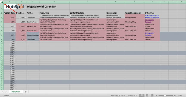
2. Select the entire table by hitting the button on the top left.
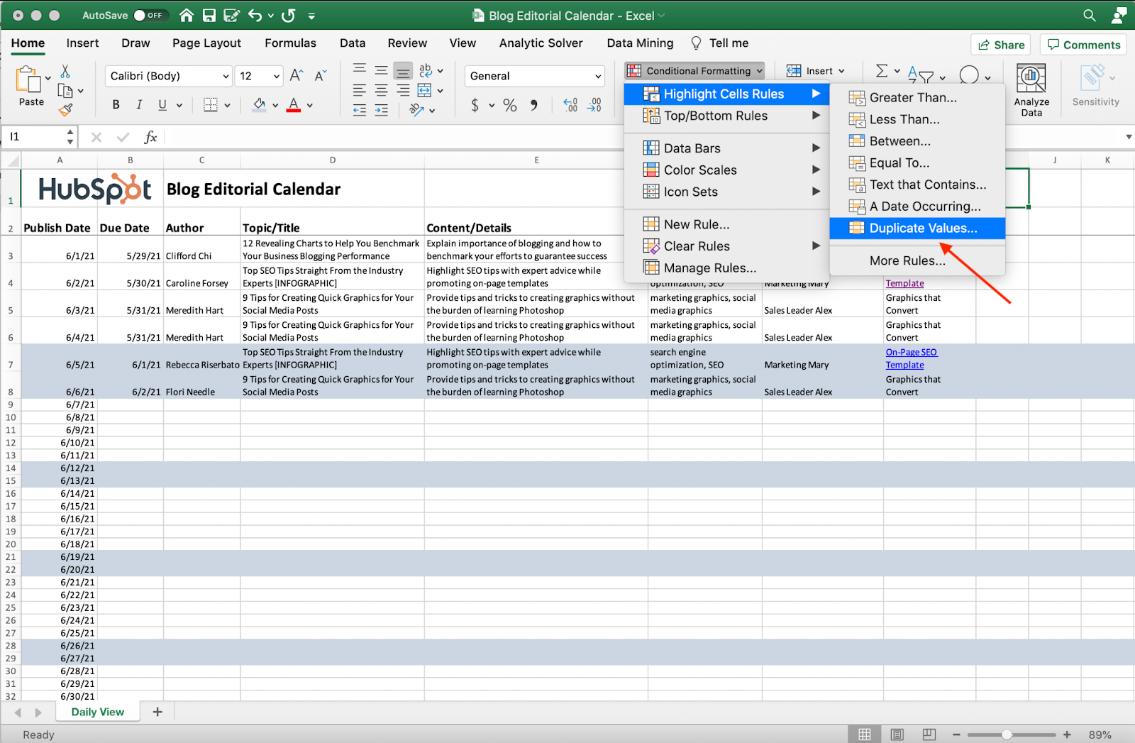
3. Click Conditional Formatting → Highlight Cells Rules → Duplicate Values.
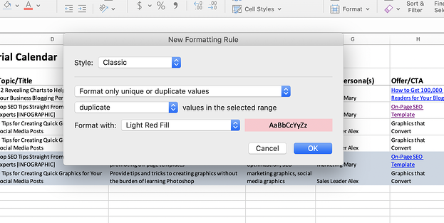
4. In the area titled “Format With”, change how you want duplicates to be highlighted. You can choose highlighting, bolding text, changing the color of text, etc.

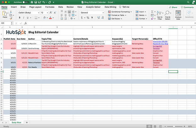
And voila. Your duplicates are now highlighted. It should look something like this:

2. Count duplicates in Excel.

Now that you've found your duplicates, you might want to count them and see how many there are, especially if you have a large dataset.

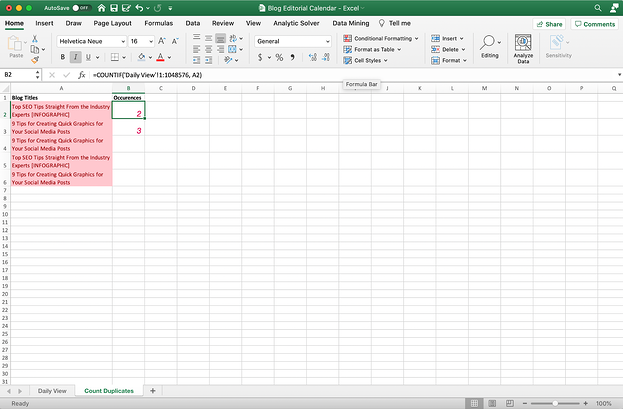
To do this, you can use this formula =COUNTIF(A:A, A2). The formula means that Excel is going to count how many times a certain value is used in a certain place.

The column A:A stands for the data table you're looking at. This will probably be a different value on your Excel sheet. Then, A2 references the value you want to count the frequency of.

To do this, follow these steps:

1. Create a new sheet in your Excel doc.

   I found that the easiest way to count duplicates in Excel is to create a new sheet in your Excel workbook.

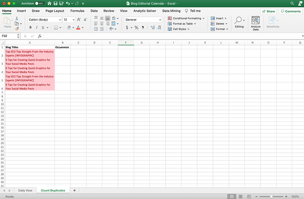
   Then, copy and paste the column that you want to count duplicates in. In the example below, I copied and pasted the blog titles from the editorial calendar to see if there were any duplicate titles.

   Then, create another column for “occurrences.” This is where we'll put the formula. Your new sheet should look something like this:

   

2. Insert the formula.

Now, you can insert the formula in the first cell under occurrences. You'll type in or copy and paste the formula. Then highlight A:A (we're going to replace this with your dataset), and click on the sheet in your Excel doc that has the data. Now, you can click on the top left to select the entire sheet, or you can just highlight the column or rows with your data.

For the second value, you'll want to go back to your second sheet, highlight the A2, and choose the value next to it on the left. In most cases, this will stay A2, A3, A4, etc.

See what this looks like in action here:

3. Remove duplicates with the remove duplicates feature.

Now it's time to remove the duplicates from your dataset.

Before you do this, I'd recommend duplicating/copying your dataset into another sheet or a whole other workbook altogether. You always want to keep your original data intact, even though you can use Excel to remove and filter the data you want. You don't want to lose data because of a wrong click.

Once you've made a copy of your data, it's time to remove the duplicates.

To remove duplicates, follow these steps:

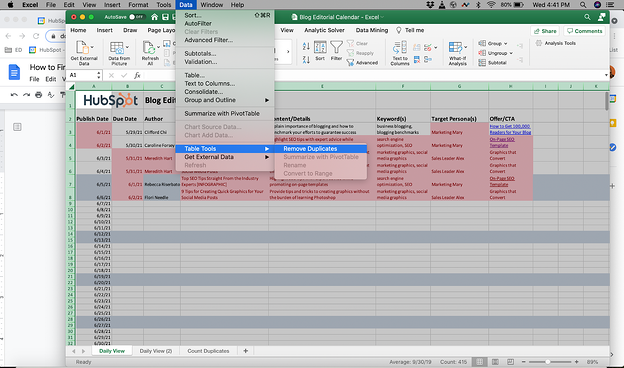
1. Select the worksheet that has duplicate values that you want to remove. Click Data → Table Tools → Remove Duplicates.
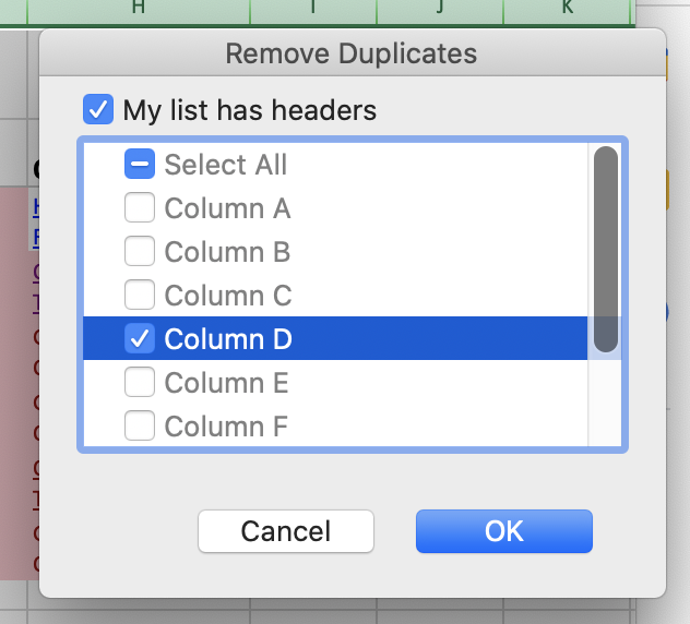
2. Choose the columns where you want to remove the duplicates.

   In this case, I only want to remove duplicate blog titles. So I'll choose column D. I kept “My list has headers” checked because there are two rows of headers before the data starts on this sheet.

   Remember that Excel will remove the entire row where the duplicate value is.

   

3. Review data.

Excel will now show you have many duplicate values were found, removed, and how many unique values remain.

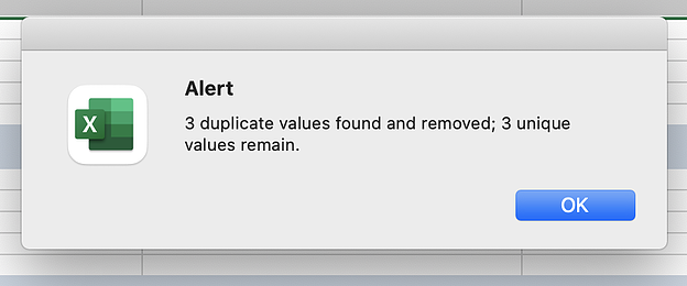
Now you can review your data. Comparing my first dataset to this dataset, you can see that all the rows containing the same blog title were deleted.

This is what the sheet used to look like:

And this is what it looks like now:

When you remove duplicates from Excel, it's important to note which column you want to remove duplicates from and remember that Excel is removing duplicates within a selected table range. You can highlight the whole workbook or you can just highlight the rows that have data in it.

Excel will automatically keep the first occurrence of the value.

Working on marketing reports or any marketing Excel sheet can leave you frustrated and banging your head against the wall (is it just me?). That's why using Excel templates and following these simple instructions on formulas can help you level up your game.