Working with large data sets is always tricky. Excel is one of the most powerful tools you can use to manipulate, format, and analyze large sets of information.

Several well-known functions exist to help you look up specific matches within a dataset, like VLookup.

But functions like VLookup had certain limitations, so Microsoft recently introduced the XLookup function to Excel. It provides a more robust method for finding specific values in a data set.

Knowing how to use it effectively can drastically cut down the time you spend trying to analyze data in Excel.

What does XLookup do in Excel?

The Benefits of XLookup in Excel

XLookup Required Arguments

XLookup Optional Arguments

How to Use XLookup in Excel

Best Practices for XLookup in Excel

What does XLookup do in Excel?

The core functionality of the XLookup is the ability to search for specific values in a range or array of data. When you run the function, a corresponding value is returned from another range or array.

Ultimately, it’s a search tool for your Excel datasets.

Depending on your arguments, XLookup will show you the first or last value in instances with more than one matching result.

Other lookup functions like VLookup (vertical lookup) or HLookup (horizontal lookup) have limitations, such as only searching from right to left. Users need to either rearrange data or find complex workarounds to mitigate this.

XLookup is a far more flexible solution, allowing you to get partial matches, use more than one search criteria and use nested queries.

Check out this XLookup Excel tutorial to see it in action:

The Benefits of XLookup in Excel

The main benefit of XLookup in Excel is the time savings it provides. You can achieve the search result without manipulating data positioning, for example.

Like other Excel lookup formulas, it saves a huge amount of time that would otherwise have to be spent manually scrolling through rows and rows of data.

When it comes to comparisons with other lookup functions, XLookup’s flexibility is key. For example, you can use wildcard characters to search for partial matches.

This helps to reduce errors overall, as you can use it to find data that may be misspelled or entered incorrectly.

The arguments for XLookup are also simpler than VLookup, making it faster and easier to use. XLookup defaults to an exact match, for example, whereas you would have to specify this in your VLookup argument.

The overall functionality of XLookup is superior since it can return multiple results at once. One example of this use case would be searching for the top five values in a particular dataset.

XLookup Required Arguments

Your XLookup function requires three arguments:

• Lookup_value: This is the value you’re searching for in an array.
• Lookup_array: This is the range of cells where you want the return value to be displayed.
• Return_array: This is the range of cells where you want the function to search for the value.

So a simple version of an XLookup would look like this:

=XLOOKUP(lookup_value, lookup_array, return_array)

XLookup Optional Arguments

The XLookup function also has several optional arguments that you can use for more complex scenarios or to narrow down your search:

• Match_mode: This determines the type of match to use, such as exact match or wildcard match to get partial matches.
• Search_mode: This determines whether your function should search from left to right or vice versa.
• If_not_found: This argument tells the function what value should be returned if there is no match at all.

With optional arguments included, the XLookup function looks like this:

=XLOOKUP(lookup_value, lookup_array, return_array, [if_not_found], [match_mode], [search_mode])

How to Use XLookup in Excel

1. Open the Excel and the datasheet on which you want to use the XLookup function.

2. Select the cell where you want to place the XLookup Excel formula.

3. Type “=” into that cell and then type “XLookup.” Click on the “XLookup” option that comes up in the dropdown.

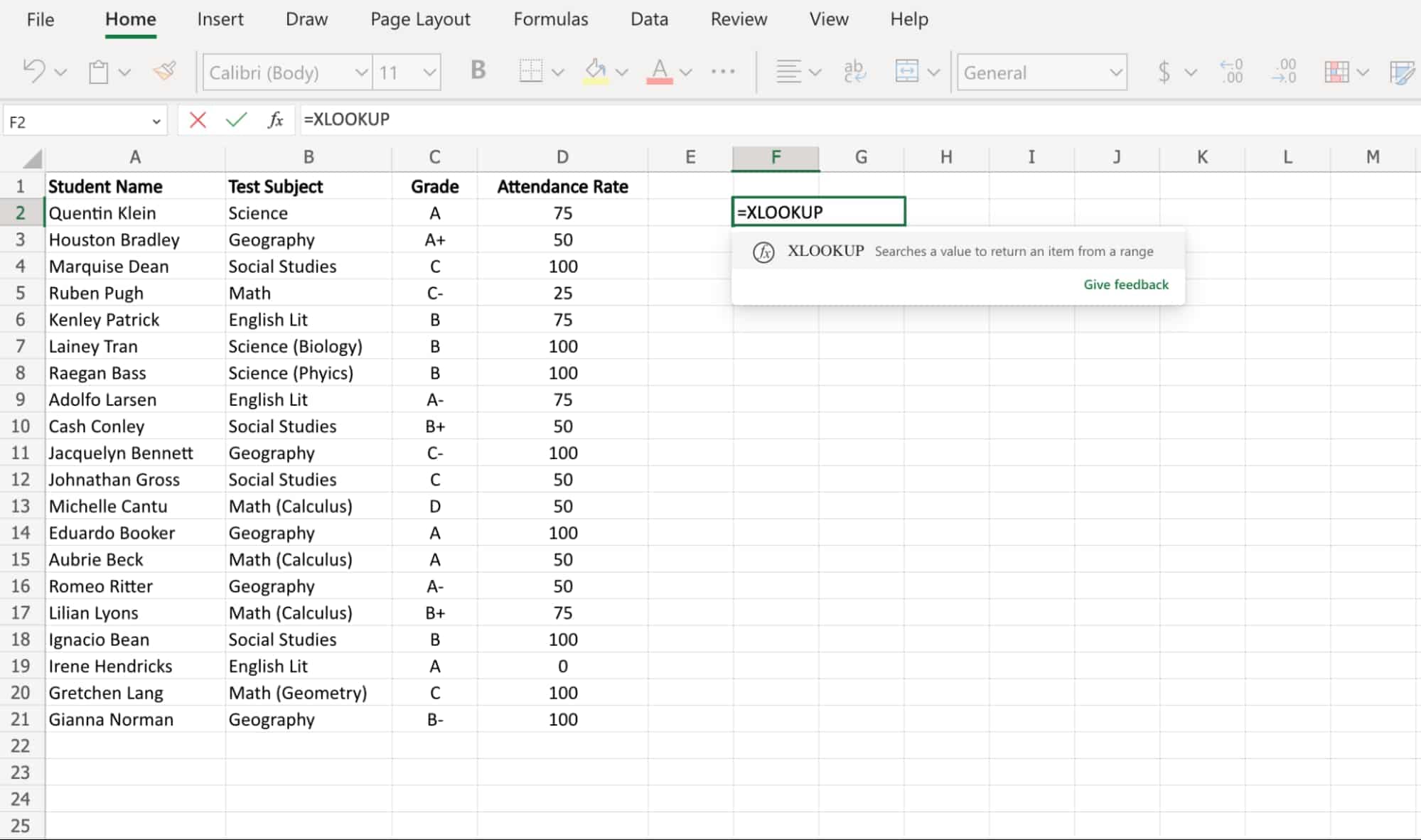
4. An opening parenthesis will automatically generate. After the opening bracket, enter the required arguments in the correct order: lookup_value, lookup_array, and return_array.

This means selecting the range of cells for each argument and placing a comma before moving on to the next argument.

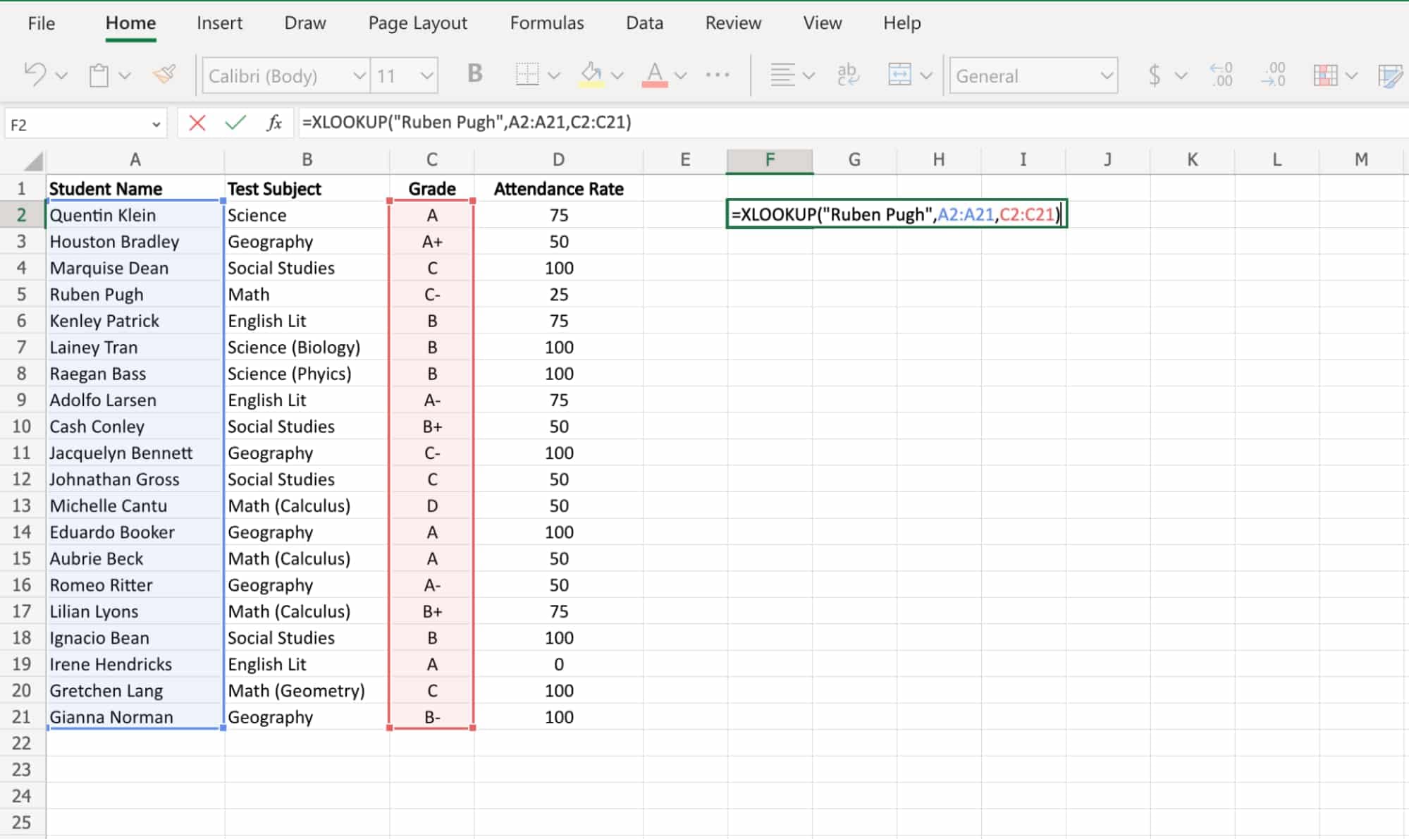
5. If you’re using any optional arguments, enter them after the required arguments.

6. When your XLookup arguments are complete, add a closing parenthesis before hitting enter.

7. The results of your XLookup should be displayed in the cell where you entered the function.

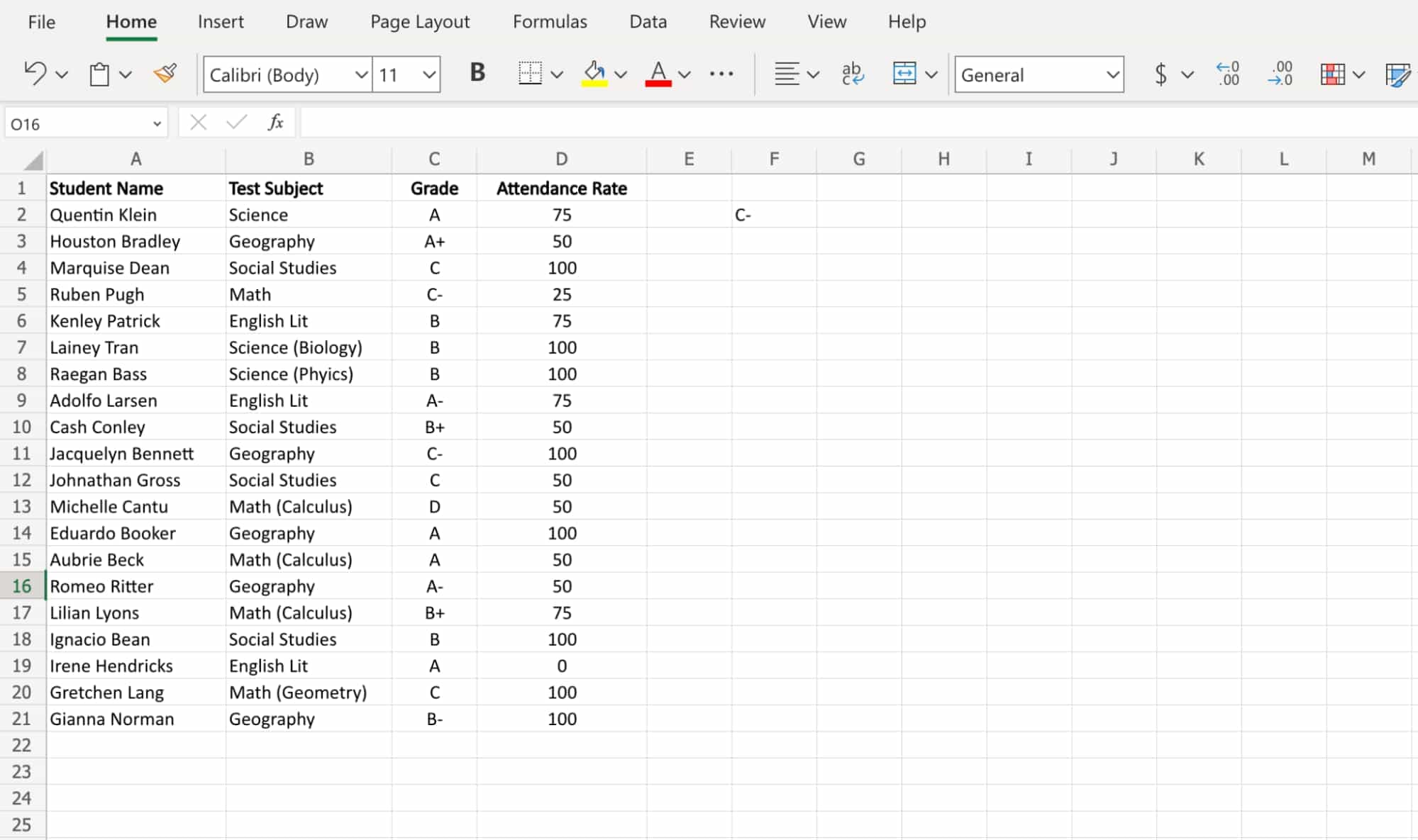In this Excel XLookup example, we used XLookup to find out the grade for a particular student. So, the lookup_value was the student's name (“Ruben Pugh”).

The lookup_array was the list of student names under column A. Finally, the lookup_return was the list of student grades under column C. With that formula, the function returned the value of the student’s grade: C-.

But how do you use XLookup with the optional arguments?

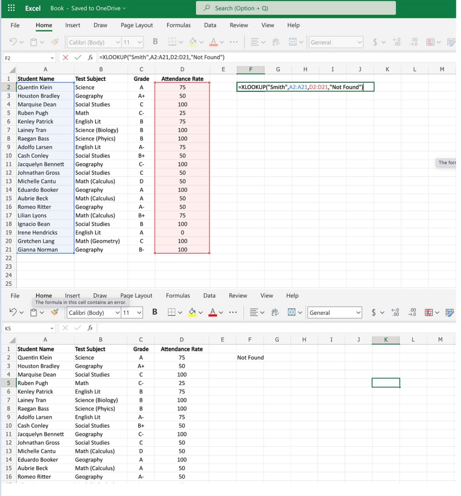
Using the same data set as above, let’s say we want to find the attendance rate for a student with the surname “Smith.”

Here, we’re telling Excel to return the message “Not Found” if it cannot retrieve the value, indicating that the student “Smith” is not on this list:

Now, let’s say we want to determine whether any students had an attendance rate of 70%. But we also want to know the next closest attendance rate if 70% does not exist in the dataset.

We’ll use the value “1” under the match_mode argument to find the next largest item if 70 does not exist:

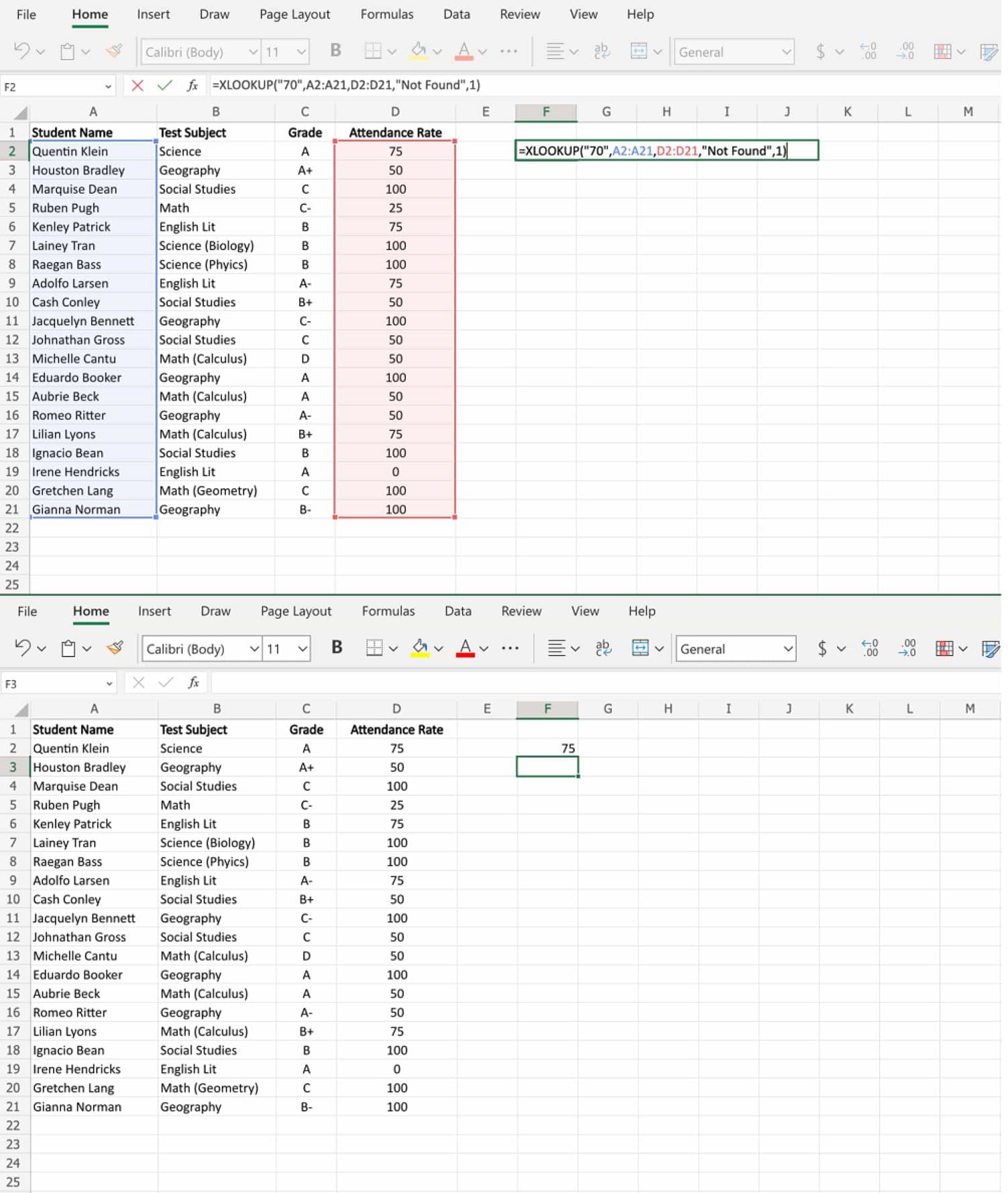Since no student has a 70% attendance rate, the XLookup has returned “75,” the next largest value.

Best Practices for XLookup in Excel

Use Descriptive References

It’s preferable to use descriptive references for the cells you’re using rather than generic ranges like A1:A12.

When it comes time to adjust your formula (which you tend to do frequently with a function like XLookup), descriptive references make it easier to understand what you were originally using the formula to do.

This is also useful if you pass the spreadsheet off to a new user who needs to understand the formula references quickly.

Use Exact Match Where Possible

Using the exact match default within the formula (as opposed to wildcard characters) helps ensure you don’t get unintended values in the return.

Wildcard characters are more useful for identifying partial matches, but the exact match is the best way to ensure the formula works as intended.

Keep Argument Ranges the Same Size

When putting your arguments together, make sure that you use the same number of cells for the return_array and the look_up array. If not, you’ll get an error, and Excel will only return #VALUE in the cell.

Test Your Formula

It’s not difficult to fix problems with a simple XLookup. But if you’re using nested functions or XLookup in conjunction with other formulas, ensure you’re testing everything along the way.

If you don’t and receive an error, it can be challenging to work backward and identify where the function is going wrong.

Getting Started

As a new and improved way to use lookup functionality in Excel, the XLookup outperforms the classic VLookup in multiple ways.

While the basics of the function are easy to grasp, it can take some practice to use XLookup in more complex ways. But with some practice data and test scenarios to work on, you’ll master the XLookup in no time.