Without freezing rows or columns in your Excel spreadsheet, everything moves when you scroll through the page, as shown in the gif below.

This can be frustrating if you can’t always see key data markers that explain what data is what, like column headers or row titles.

As with many things on Excel, there are tricks that help you make your spreadsheets easier to read, like the freeze function. In this post, learn how to freeze rows and columns in Excel to ensure that, when you scroll around, you’ll always be able to view the key data points that matter most.

How to Freeze a Top Row in Excel

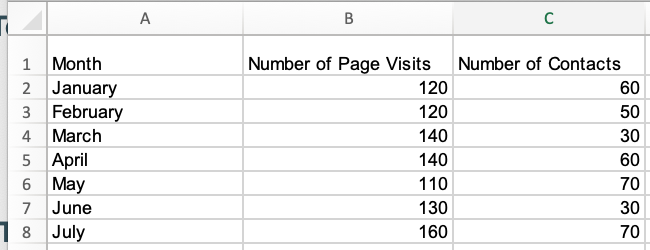
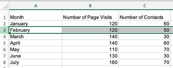
The image below is the sample data set I’ll use to run through the explanations in this piece.

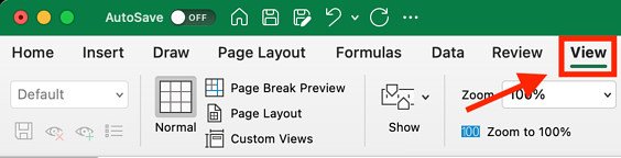
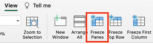
1. To freeze the top row in an Excel spreadsheet, navigate to the header toolbar and select
View, as shown in the image below.



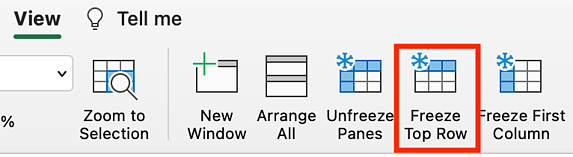
2. When the
View menu options appear, Click
Freeze Top Row, outlined in red in the image below.  

Once selected, everything in the top row of your Excel spreadsheet (row 1) will be frozen, and you can scroll up and down in your spreadsheet, but the top rows won’t move, as shown in the gif below.

How to Freeze a Specific Row in Excel

While excel has native functions for freezing the top row of a data set and the first column of a data set, there are additional steps to take to freeze other elements of your data set that aren’t those two things.

1. To freeze a specific row in Excel, select the row number immediately underneath the one you want frozen. For this example, I’m selecting row number three to freeze row number two.

2. After selecting your row, navigate to View in the header toolbar and select Freeze Panes.

Once selected, you’ll be able to scroll up and down through your spreadsheet and always see row two.

Note that using the Freeze Panes function to freeze rows also freezes every row above the row you initially selected. For example, in the gif below, I selected row five which also freeze rows four, three, two, and one.

How to Freeze the First Column in Excel

1. To freeze the first column of your Excel spreadsheet (column A), navigate to the Excel header toolbar, select View, and click Freeze First Column.

Once selected, you’ll be able to scroll side to side within your sheet, and the first column of your data set will always be visible, as shown in the image below.

How to Freeze a Specific Column in Excel

1. If you want to freeze a specific column in excel, select the column letter that is immediately next to the column you want frozen and click Freeze Panes in the View header menu.

Once selected, you can scroll side to side through your entire data set and continue to see those columns. In the gif below, I’ve frozen columns A and B.

Using the freeze function in Excel makes your spreadsheets easier to understand, as you can ensure that critical rows and columns are always visible as you scroll through your data.